Streamlines are paths that are always tangential to a vector field. In the case of a steady field, it's identical to the path of a massless particle that moves with the "flow".
geom_streamline(
  mapping = NULL,
  data = NULL,
  stat = "streamline",
  position = "identity",
  ...,
  L = 5,
  min.L = 0,
  res = 1,
  S = NULL,
  dt = NULL,
  xwrap = NULL,
  ywrap = NULL,
  skip = 1,
  skip.x = skip,
  skip.y = skip,
  n = NULL,
  nx = n,
  ny = n,
  jitter = 1,
  jitter.x = jitter,
  jitter.y = jitter,
  arrow.angle = 6,
  arrow.length = 0.5,
  arrow.ends = "last",
  arrow.type = "closed",
  arrow = grid::arrow(arrow.angle, grid::unit(arrow.length, "lines"), ends = arrow.ends,
    type = arrow.type),
  lineend = "butt",
  na.rm = TRUE,
  show.legend = NA,
  inherit.aes = TRUE
)

stat_streamline(
  mapping = NULL,
  data = NULL,
  geom = "streamline",
  position = "identity",
  ...,
  L = 5,
  min.L = 0,
  res = 1,
  S = NULL,
  dt = NULL,
  xwrap = NULL,
  ywrap = NULL,
  skip = 1,
  skip.x = skip,
  skip.y = skip,
  n = NULL,
  nx = n,
  ny = n,
  jitter = 1,
  jitter.x = jitter,
  jitter.y = jitter,
  arrow.angle = 6,
  arrow.length = 0.5,
  arrow.ends = "last",
  arrow.type = "closed",
  arrow = grid::arrow(arrow.angle, grid::unit(arrow.length, "lines"), ends = arrow.ends,
    type = arrow.type),
  lineend = "butt",
  na.rm = TRUE,
  show.legend = NA,
  inherit.aes = TRUE
)
Arguments
- mapping
Set of aesthetic mappings created by
aes(). If specified andinherit.aes = TRUE(the default), it is combined with the default mapping at the top level of the plot. You must supplymappingif there is no plot mapping.- data
The data to be displayed in this layer. There are three options:
If
NULL, the default, the data is inherited from the plot data as specified in the call toggplot().A
data.frame, or other object, will override the plot data. All objects will be fortified to produce a data frame. Seefortify()for which variables will be created.A
functionwill be called with a single argument, the plot data. The return value must be adata.frame, and will be used as the layer data. Afunctioncan be created from aformula(e.g.~ head(.x, 10)).- stat
The statistical transformation to use on the data for this layer, either as a
ggprotoGeomsubclass or as a string naming the stat stripped of thestat_prefix (e.g."count"rather than"stat_count")- position
Position adjustment, either as a string naming the adjustment (e.g.
"jitter"to useposition_jitter), or the result of a call to a position adjustment function. Use the latter if you need to change the settings of the adjustment.- ...
Other arguments passed on to
layer(). These are often aesthetics, used to set an aesthetic to a fixed value, likecolour = "red"orsize = 3. They may also be parameters to the paired geom/stat.- L,
typical length of a streamline in x and y units
- min.L
minimum length of segments to show
- res,
resolution parameter (higher numbers increases the resolution)
- S
optional numeric number of timesteps for integration
- dt
optional numeric size "timestep" for integration
- xwrap, ywrap
vector of length two used to wrap the circular dimension.
- skip, skip.x, skip.y
numeric specifying number of gridpoints not to draw in the x and y direction
- n, nx, ny
optional numeric indicating the number of points to draw in the x and y direction (replaces
skipif notNULL)- jitter, jitter.x, jitter.y
amount of jitter of the starting points
- arrow.length, arrow.angle, arrow.ends, arrow.type
parameters passed to grid::arrow
- arrow
specification for arrow heads, as created by
grid::arrow().- lineend
Line end style (round, butt, square).
- na.rm
If
FALSE, the default, missing values are removed with a warning. IfTRUE, missing values are silently removed.- show.legend
logical. Should this layer be included in the legends?
NA, the default, includes if any aesthetics are mapped.FALSEnever includes, andTRUEalways includes. It can also be a named logical vector to finely select the aesthetics to display.- inherit.aes
If
FALSE, overrides the default aesthetics, rather than combining with them. This is most useful for helper functions that define both data and aesthetics and shouldn't inherit behaviour from the default plot specification, e.g.borders().- geom
The geometric object to use to display the data, either as a
ggprotoGeomsubclass or as a string naming the geom stripped of thegeom_prefix (e.g."point"rather than"geom_point")
Details
Streamlines are computed by simple integration with a forward Euler method.
By default, stat_streamline() computes dt and S from L, res,
the resolution of the grid and the mean magnitude of the field. S is
then defined as the number of steps necessary to make a streamline of length
L under an uniform mean field and dt is chosen so that each step is no
larger than the resolution of the data (divided by the res parameter). Be
aware that this rule of thumb might fail in field with very skewed distribution
of magnitudes.
Alternatively, L and/or res are ignored if S and/or dt are specified
explicitly. This not only makes it possible to fine-tune the result but also
divorces the integration parameters from the properties of the data and makes
it possible to compare streamlines between different fields.
The starting grid is a semi regular grid defined, either by the resolution of the
field and the skip.x and skip.y parameters o the nx and ny parameters,
jittered by an amount proportional to the resolution of the data and the
jitter.x and jitter.y parameters.
It might be important that the units of the vector field are compatible to the units
of the x and y dimensions. For example, passing dx and dy in m/s on a
longitude-latitude grid will might misleading results (see spherical).
Missing values are not permitted and the field must be defined on a regular grid, for now.
Aesthetics
stat_streamline understands the following aesthetics (required aesthetics are in bold)
x
y
dx
dy
alphacolourlinetypesize
Computed variables
- step
step in the simulation
- dx
dx at each location of the streamline
- dy
dy at each location of the streamline
See also
Other ggplot2 helpers:
DivideTimeseries(),
MakeBreaks(),
WrapCircular(),
geom_arrow(),
geom_contour2(),
geom_contour_fill(),
geom_label_contour(),
geom_relief(),
guide_colourstrip(),
map_labels,
reverselog_trans(),
scale_divergent,
scale_longitude,
stat_na(),
stat_subset()
Examples
library(data.table)
library(ggplot2)
data(geopotential)
geopotential <- copy(geopotential)[date == date[1]]
geopotential[, gh.z := Anomaly(gh), by = .(lat)]
#> lon lat lev gh date gh.z
#> 1: 0.0 -22.5 700 3163.839 1990-01-01 13.67219
#> 2: 2.5 -22.5 700 3162.516 1990-01-01 12.34968
#> 3: 5.0 -22.5 700 3162.226 1990-01-01 12.05939
#> 4: 7.5 -22.5 700 3162.323 1990-01-01 12.15607
#> 5: 10.0 -22.5 700 3163.097 1990-01-01 12.93024
#> ---
#> 4028: 347.5 -90.0 700 2715.936 1990-01-01 0.00000
#> 4029: 350.0 -90.0 700 2715.936 1990-01-01 0.00000
#> 4030: 352.5 -90.0 700 2715.936 1990-01-01 0.00000
#> 4031: 355.0 -90.0 700 2715.936 1990-01-01 0.00000
#> 4032: 357.5 -90.0 700 2715.936 1990-01-01 0.00000
geopotential[, c("u", "v") := GeostrophicWind(gh.z, lon, lat)]
#> lon lat lev gh date gh.z u v
#> 1: 0.0 -22.5 700 3163.839 1990-01-01 13.67219 NA 1.08181190
#> 2: 2.5 -22.5 700 3162.516 1990-01-01 12.34968 NA 0.55189199
#> 3: 5.0 -22.5 700 3162.226 1990-01-01 12.05939 NA 0.06625043
#> 4: 7.5 -22.5 700 3162.323 1990-01-01 12.15607 NA -0.29800162
#> 5: 10.0 -22.5 700 3163.097 1990-01-01 12.93024 NA -0.75064329
#> ---
#> 4028: 347.5 -90.0 700 2715.936 1990-01-01 0.00000 NA 0.00000000
#> 4029: 350.0 -90.0 700 2715.936 1990-01-01 0.00000 NA 0.00000000
#> 4030: 352.5 -90.0 700 2715.936 1990-01-01 0.00000 NA 0.00000000
#> 4031: 355.0 -90.0 700 2715.936 1990-01-01 0.00000 NA 0.00000000
#> 4032: 357.5 -90.0 700 2715.936 1990-01-01 0.00000 NA 0.00000000
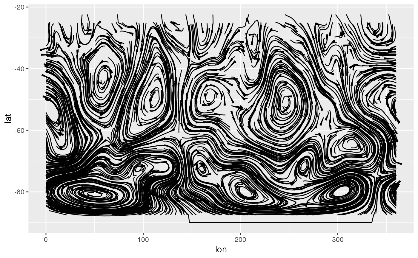
(g <- ggplot(geopotential, aes(lon, lat)) +
geom_contour2(aes(z = gh.z), xwrap = c(0, 360)) +
geom_streamline(aes(dx = dlon(u, lat), dy = dlat(v)), L = 60,
xwrap = c(0, 360)))
#> Warning: 'xwrap' and 'ywrap' will be deprecated. Use ggperiodic::periodic insead.
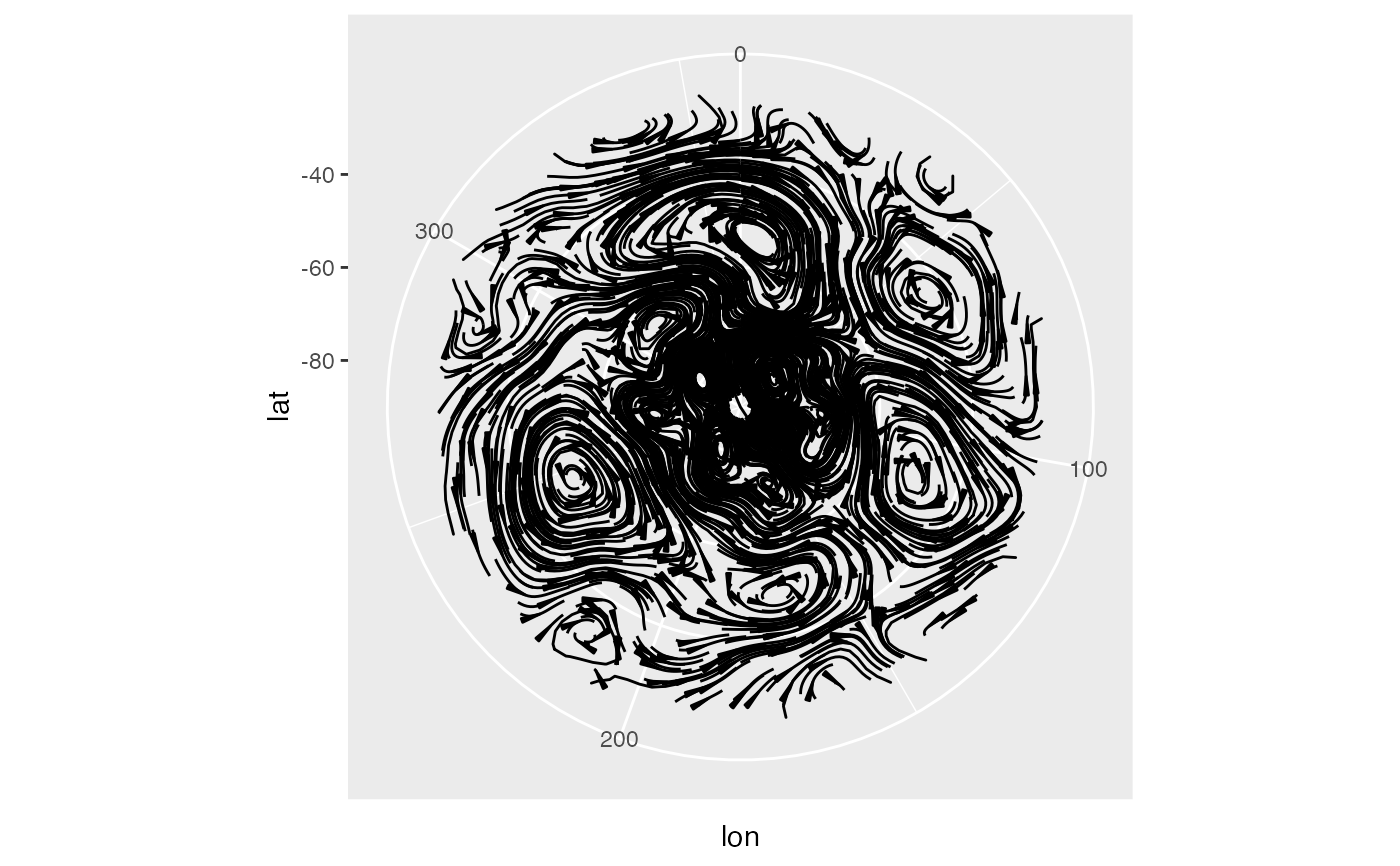
 # The circular parameter is particularly important for polar coordinates
g + coord_polar()
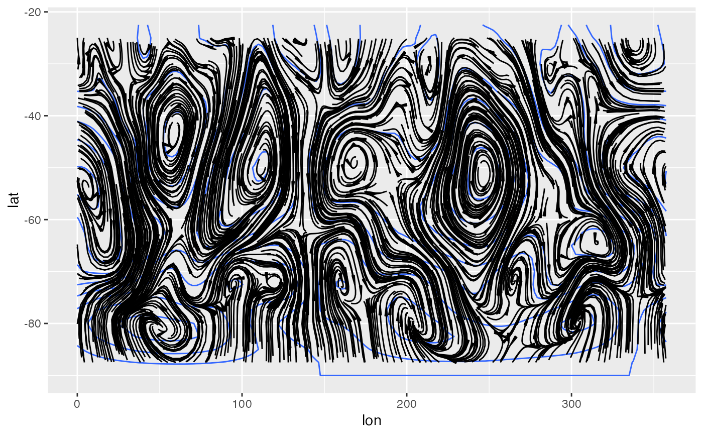
 # If u and v are not converted into degrees/second, the resulting
# streamlines have problems, specially near the pole.
ggplot(geopotential, aes(lon, lat)) +
geom_contour(aes(z = gh.z)) +
geom_streamline(aes(dx = u, dy = v), L = 50)
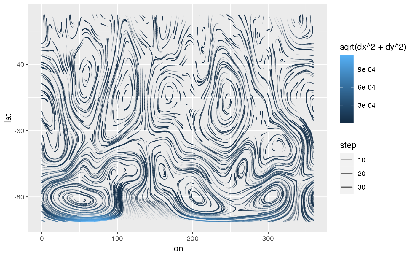
 # The step variable can be mapped to size or alpha to
# get cute "drops". It's important to note that ..dx.. (the calculated variable)
# is NOT the same as dx (from the data).
ggplot(geopotential, aes(lon, lat)) +
geom_streamline(aes(dx = dlon(u, lat), dy = dlat(v), alpha = ..step..,
color = sqrt(..dx..^2 + ..dy..^2), size = ..step..),
L = 40, xwrap = c(0, 360), res = 2, arrow = NULL,
lineend = "round") +
scale_size(range = c(0, 0.6))
 # Using topographic information to simulate "rivers" from slope
topo <- GetTopography(295, -55+360, -30, -42, res = 1/20) # needs internet!
topo[, c("dx", "dy") := Derivate(h ~ lon + lat)]
#> lon lat h dx dy
#> 1: 295.025 -30.025 178 NA NA
#> 2: 295.075 -30.025 180 -10 NA
#> 3: 295.125 -30.025 177 -30 NA
#> 4: 295.175 -30.025 177 -10 NA
#> 5: 295.225 -30.025 176 10 NA
#> ---
#> 47996: 304.775 -41.975 -4525 -530 NA
#> 47997: 304.825 -41.975 -4589 -2270 NA
#> 47998: 304.875 -41.975 -4752 -2100 NA
#> 47999: 304.925 -41.975 -4799 -760 NA
#> 48000: 304.975 -41.975 -4828 NA NA
topo[h <= 0, c("dx", "dy") := 0]
#> lon lat h dx dy
#> 1: 295.025 -30.025 178 NA NA
#> 2: 295.075 -30.025 180 -10 NA
#> 3: 295.125 -30.025 177 -30 NA
#> 4: 295.175 -30.025 177 -10 NA
#> 5: 295.225 -30.025 176 10 NA
#> ---
#> 47996: 304.775 -41.975 -4525 0 0
#> 47997: 304.825 -41.975 -4589 0 0
#> 47998: 304.875 -41.975 -4752 0 0
#> 47999: 304.925 -41.975 -4799 0 0
#> 48000: 304.975 -41.975 -4828 0 0
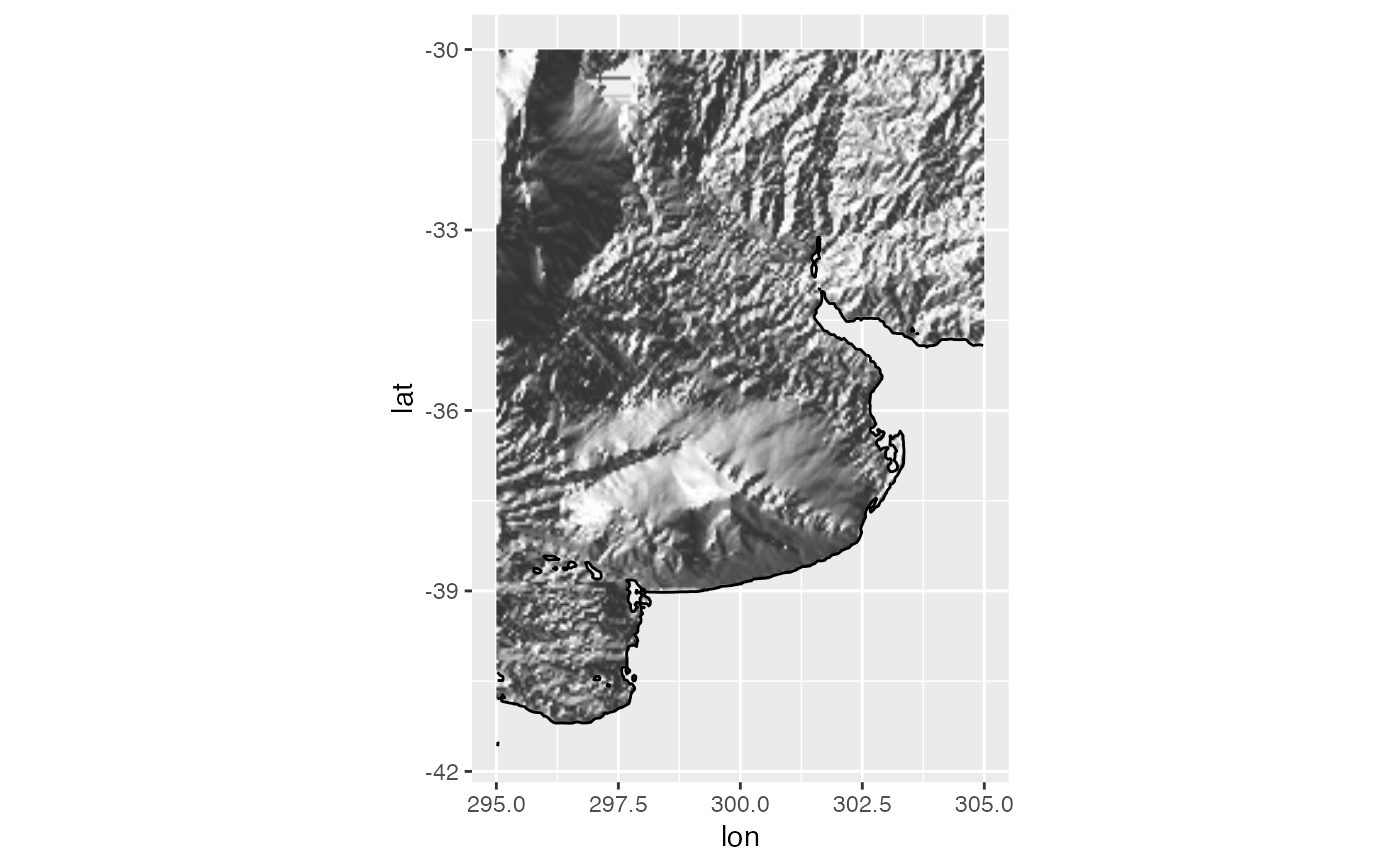
# See how in this example the integration step is too coarse in the
# western montanous region where the slope is much higher than in the
# flatlands of La Pampa at in the east.
ggplot(topo, aes(lon, lat)) +
geom_relief(aes(z = h), interpolate = TRUE, data = topo[h >= 0]) +
geom_contour(aes(z = h), breaks = 0, color = "black") +
geom_streamline(aes(dx = -dx, dy = -dy), L = 10, skip = 3, arrow = NULL,
color = "#4658BD") +
coord_quickmap()
#> Warning: Computation failed in `stat_streamline()`
#> Caused by error:
#> ! 'x' and 'y' do not define a regular grid.
