Filled 2d contours of a 3d surface

While ggplot2's geom_contour can plot nice contours, it doesn't work with the polygon geom. This stat makes some small manipulation of the data to ensure that all contours are closed and also computes a new aesthetic int.level, which differs from level (computed by ggplot2::geom_contour) in that represents the value of the z aesthetic inside the contour instead of at the edge. It also computes breaks globally instead of per panel, so that faceted plots have all the same binwidth.

geom_contour_fill(
  mapping = NULL,
  data = NULL,
  stat = "ContourFill",
  position = "identity",
  ...,
  breaks = MakeBreaks(),
  bins = NULL,
  binwidth = NULL,
  kriging = FALSE,
  global.breaks = TRUE,
  na.fill = FALSE,
  show.legend = NA,
  inherit.aes = TRUE
)

stat_contour_fill(
  mapping = NULL,
  data = NULL,
  geom = "polygon",
  position = "identity",
  ...,
  breaks = MakeBreaks(),
  bins = NULL,
  binwidth = NULL,
  global.breaks = TRUE,
  kriging = FALSE,
  na.fill = FALSE,
  show.legend = NA,
  inherit.aes = TRUE
)

Arguments

mapping

Set of aesthetic mappings created by aes(). If specified and inherit.aes = TRUE (the default), it is combined with the default mapping at the top level of the plot. You must supply mapping if there is no plot mapping.

data

The data to be displayed in this layer. There are three options:

If NULL, the default, the data is inherited from the plot data as specified in the call to ggplot().

A data.frame, or other object, will override the plot data. All objects will be fortified to produce a data frame. See fortify() for which variables will be created.

A function will be called with a single argument, the plot data. The return value must be a data.frame, and will be used as the layer data. A function can be created from a formula (e.g. ~ head(.x, 10)).

stat

The statistical transformation to use on the data for this layer, either as a ggproto Geom subclass or as a string naming the stat stripped of the stat_ prefix (e.g. "count" rather than "stat_count")

position

Position adjustment, either as a string naming the adjustment (e.g. "jitter" to use position_jitter), or the result of a call to a position adjustment function. Use the latter if you need to change the settings of the adjustment.

...

Other arguments passed on to layer(). These are often aesthetics, used to set an aesthetic to a fixed value, like colour = "red" or size = 3. They may also be parameters to the paired geom/stat.

breaks

numeric vector of breaks

bins

Number of evenly spaced breaks.

binwidth

Distance between breaks.

kriging

Logical indicating whether to perform ordinary kriging before contouring. Use this if you want to use contours with irregularly spaced data.

global.breaks

Logical indicating whether breaks should be computed for the whole data or for each grouping.

na.fill

How to fill missing values.

• FALSE for letting the computation fail with no interpolation

• TRUE for imputing missing values with Impute2D

• A numeric value for constant imputation

• A function that takes a vector and returns a numeric (e.g. mean)

show.legend

logical. Should this layer be included in the legends? NA, the default, includes if any aesthetics are mapped. FALSE never includes, and TRUE always includes. It can also be a named logical vector to finely select the aesthetics to display.

inherit.aes

If FALSE, overrides the default aesthetics, rather than combining with them. This is most useful for helper functions that define both data and aesthetics and shouldn't inherit behaviour from the default plot specification, e.g. borders().

geom

The geometric object to use to display the data, either as a ggproto Geom subclass or as a string naming the geom stripped of the geom_ prefix (e.g. "point" rather than "geom_point")

Aesthetics

geom_contour_fill understands the following aesthetics (required aesthetics are in bold):

• x

• y

• alpha

• colour

• group

• linetype

• size

• weight

Computed variables

level

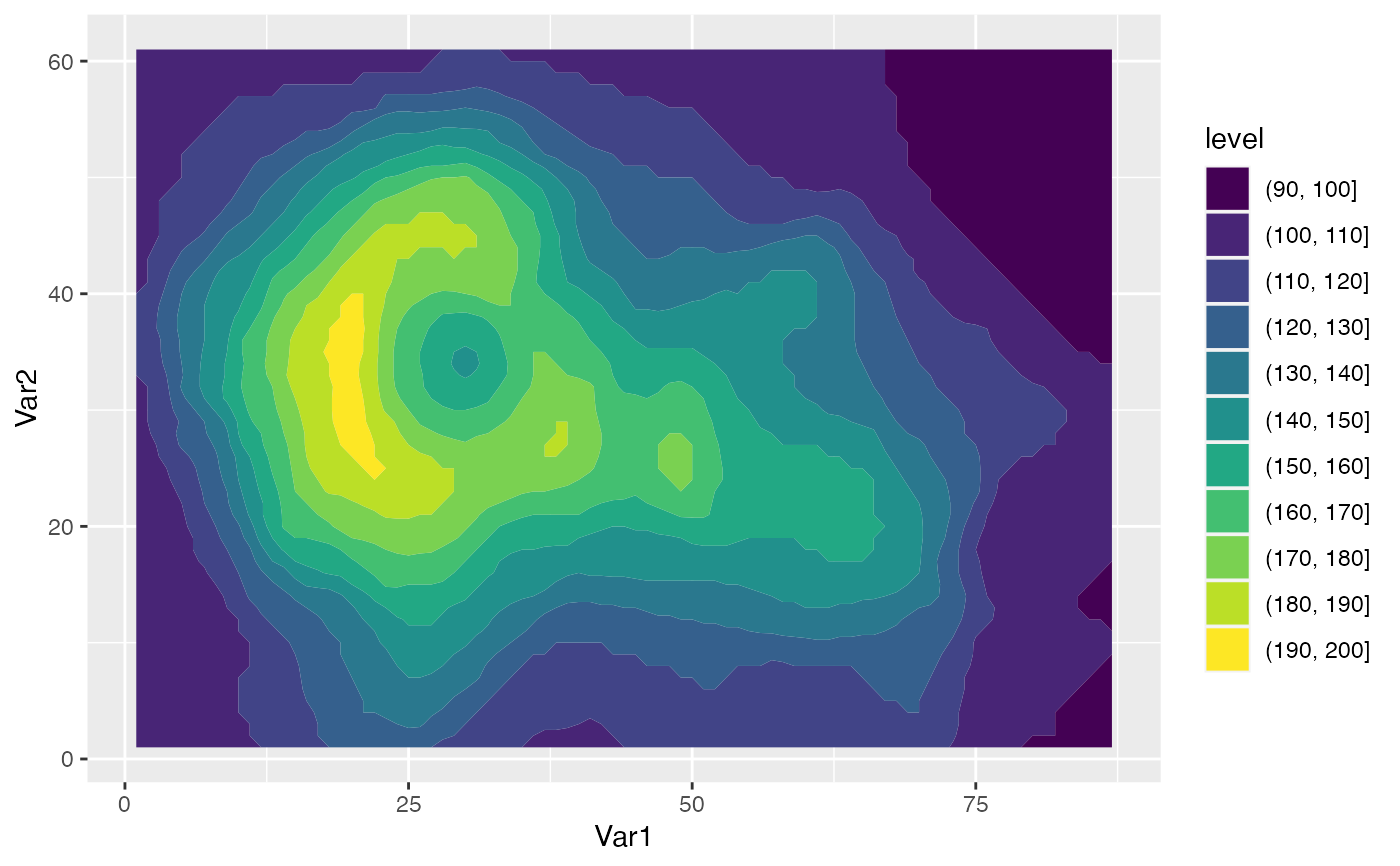
An ordered factor that represents bin ranges.

level_d

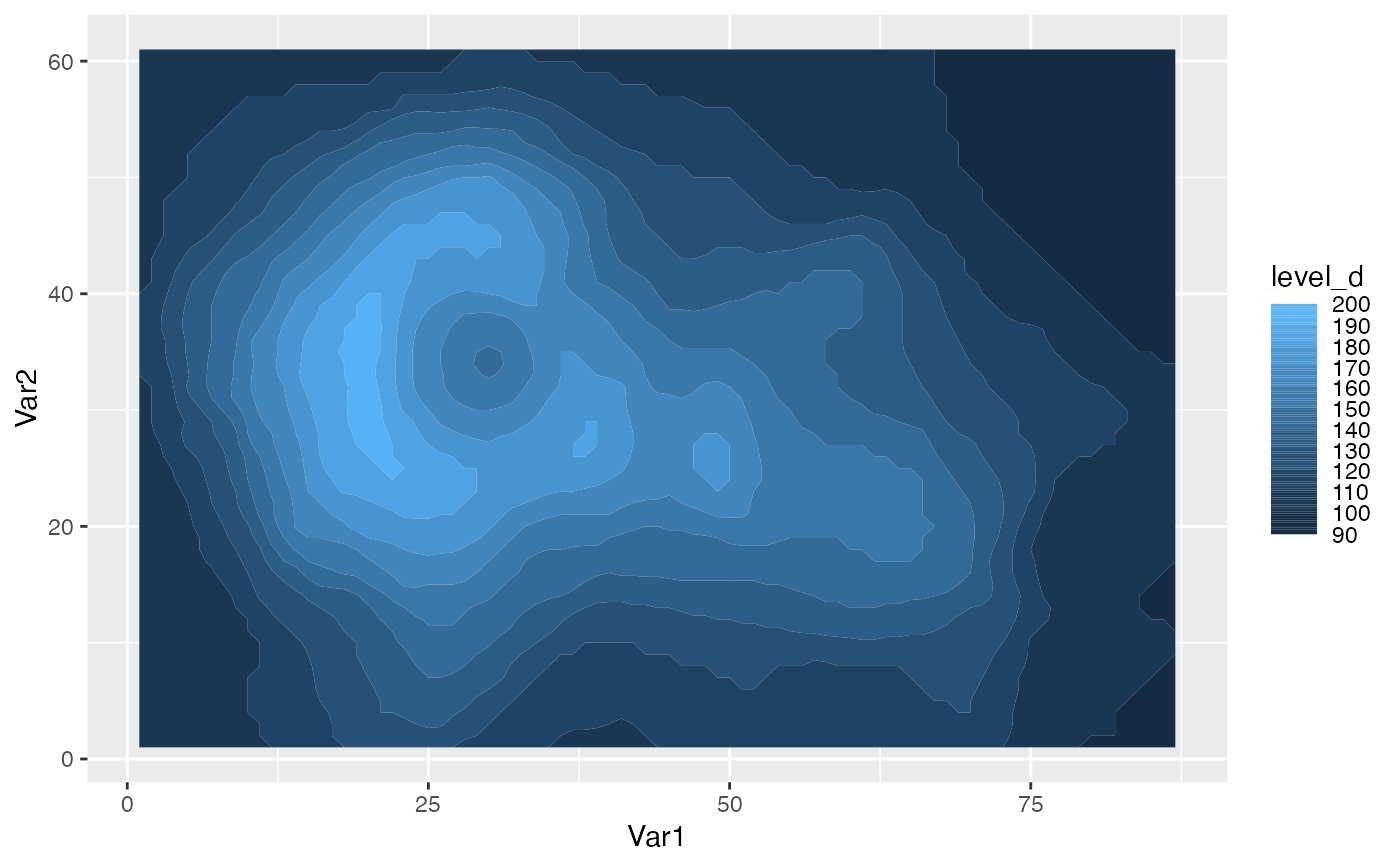
Same as level, but automatically uses scale_fill_discretised()

level_low,level_high,level_mid

Lower and upper bin boundaries for each band, as well the mid point between the boundaries.

See also

Other ggplot2 helpers: DivideTimeseries(), MakeBreaks(), WrapCircular(), geom_arrow(), geom_contour2(), geom_label_contour(), geom_relief(), geom_streamline(), guide_colourstrip(), map_labels, reverselog_trans(), scale_divergent, scale_longitude, stat_na(), stat_subset()

Examples

library(ggplot2)
surface <- reshape2::melt(volcano)
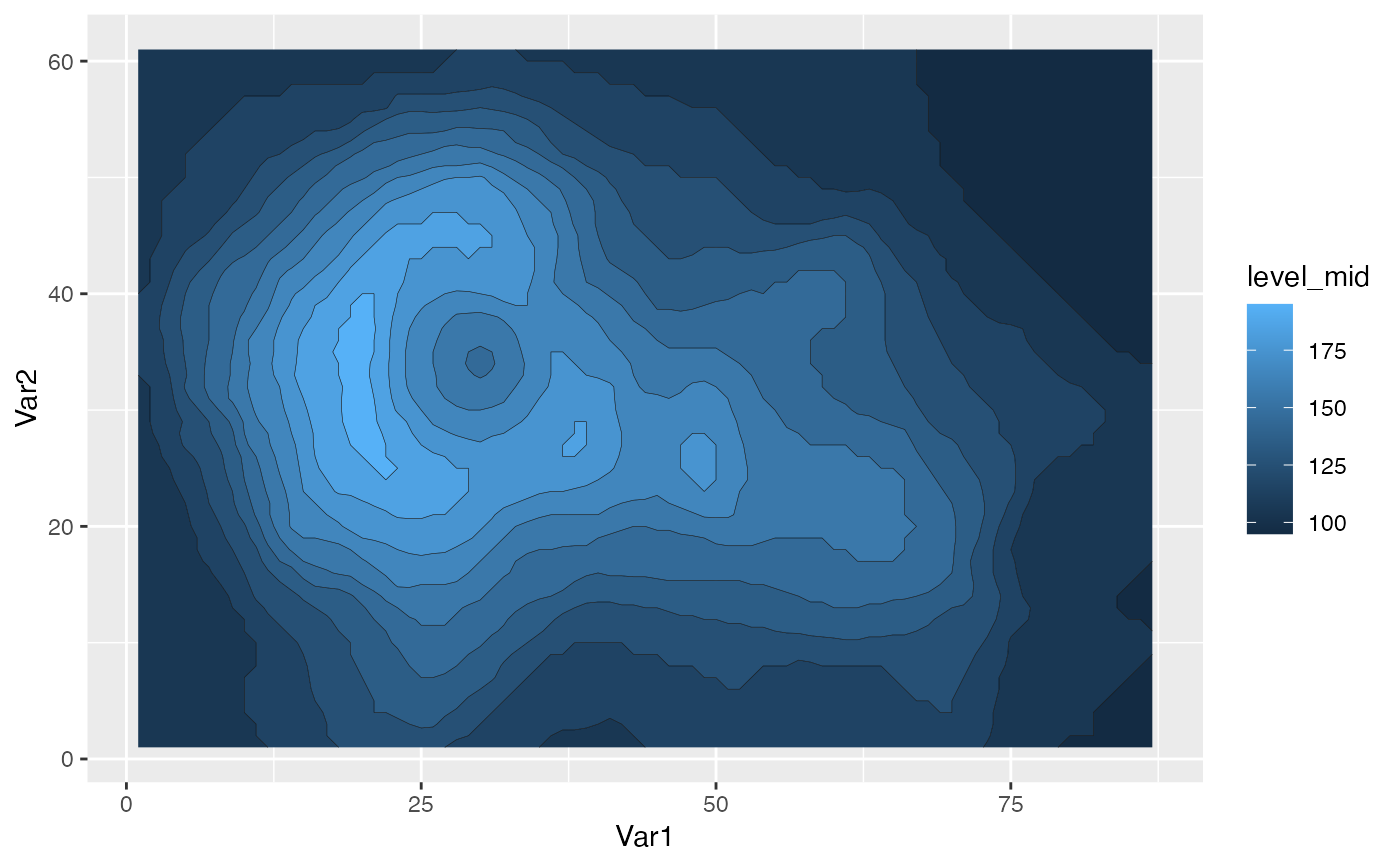
ggplot(surface, aes(Var1, Var2, z = value)) +
  geom_contour_fill() +
  geom_contour(color = "black", size = 0.1)
#> Warning: Using `size` aesthetic for lines was deprecated in ggplot2 3.4.0.
#> ℹ Please use `linewidth` instead.


ggplot(surface, aes(Var1, Var2, z = value)) +
  geom_contour_fill(aes(fill = stat(level)))


ggplot(surface, aes(Var1, Var2, z = value)) +
  geom_contour_fill(aes(fill = stat(level_d)))