Derivate a discrete variable using finite differences

Derivate a discrete variable using finite differences

Derivate(
  formula,
  order = 1,
  cyclical = FALSE,
  fill = FALSE,
  data = NULL,
  sphere = FALSE,
  a = 6371000,
  equispaced = TRUE
)

Laplacian(
  formula,
  cyclical = FALSE,
  fill = FALSE,
  data = NULL,
  sphere = FALSE,
  a = 6371000,
  equispaced = TRUE
)

Divergence(
  formula,
  cyclical = FALSE,
  fill = FALSE,
  data = NULL,
  sphere = FALSE,
  a = 6371000,
  equispaced = TRUE
)

Vorticity(
  formula,
  cyclical = FALSE,
  fill = FALSE,
  data = NULL,
  sphere = FALSE,
  a = 6371000,
  equispaced = TRUE
)

Arguments

formula

a formula indicating dependent and independent variables

order

order of the derivative

cyclical

logical vector of boundary condition for each independent variable

fill

logical indicating whether to fill values at the boundaries with forward and backwards differencing

data

optional data.frame containing the variables

sphere

logical indicating whether to use spherical coordinates (see details)

a

radius to use in spherical coordinates (defaults to Earth's radius)

equispaced

logical indicating whether points are equispaced or not.

Value

If there is one independent variable and one dependent variable, a numeric vector of the same length as the dependent variable. If there are two or more independent variables or two or more dependent variables, a list containing the directional derivatives of each dependent variables.

Details

Each element of the return vector is an estimation of \(\frac{\partial^n x}{\partial y^{n}}\) by centred finite differences.

If sphere = TRUE, then the first two independent variables are assumed to be longitude and latitude (in that order) in degrees. Then, a correction is applied to the derivative so that they are in the same units as a.

Using fill = TRUE will degrade the solution near the edges of a non-cyclical boundary. Use with caution.

Laplacian(), Divergence() and Vorticity() are convenient wrappers that call Derivate() and make the appropriate sums. For Divergence() and Vorticity(), formula must be of the form vx + vy ~ x + y (in that order).

See also

Other meteorology functions: EOF(), GeostrophicWind(), WaveFlux(), thermodynamics, waves

Examples

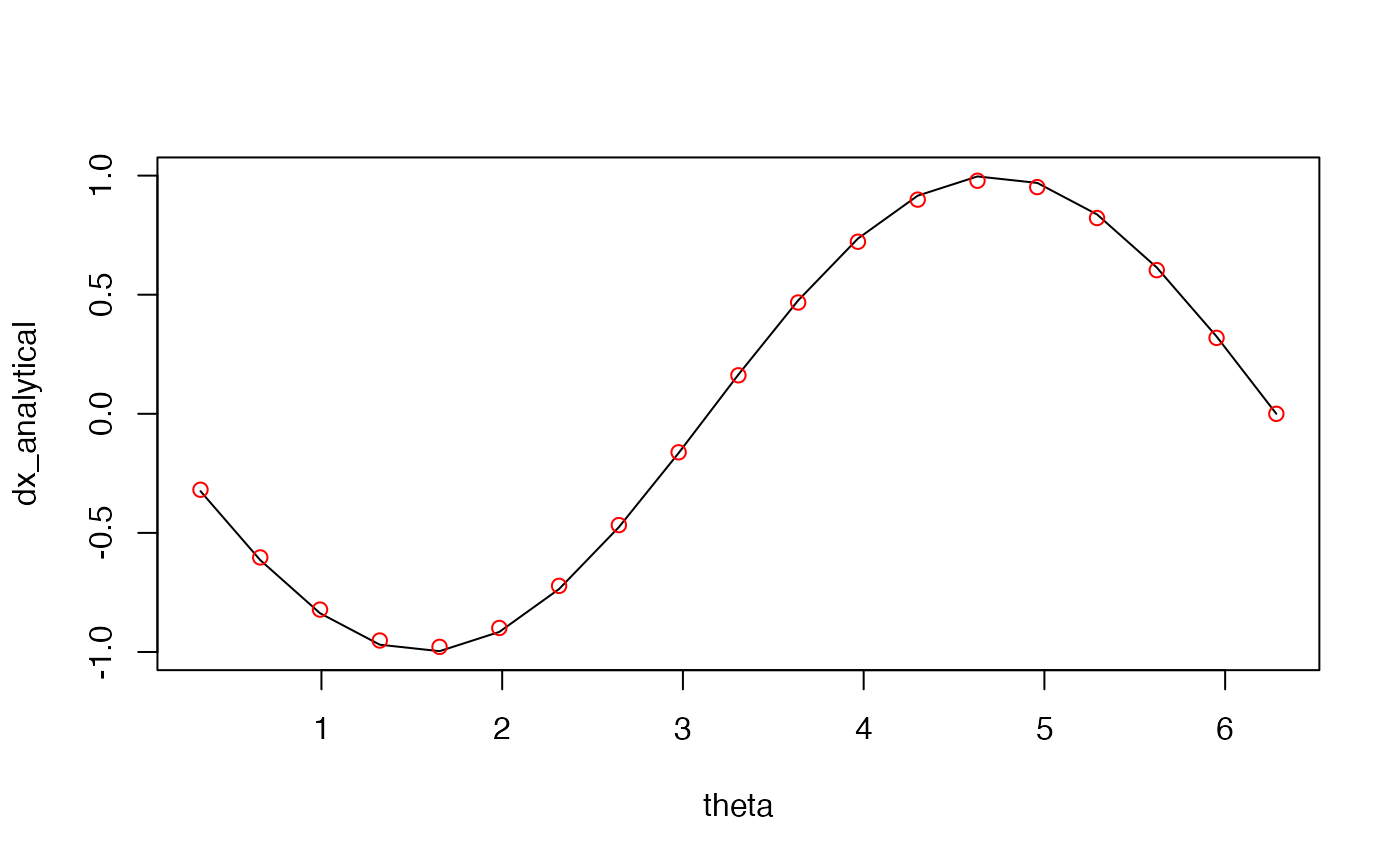
theta <- seq(0, 360, length.out = 20)*pi/180
theta <- theta[-1]
x <- cos(theta)
dx_analytical <- -sin(theta)
dx_finitediff <- Derivate(x ~ theta, cyclical = TRUE)[[1]]

plot(theta, dx_analytical, type = "l")
points(theta, dx_finitediff, col = "red")


# Curvature (Laplacian)
# Note the different boundary conditions for each dimension
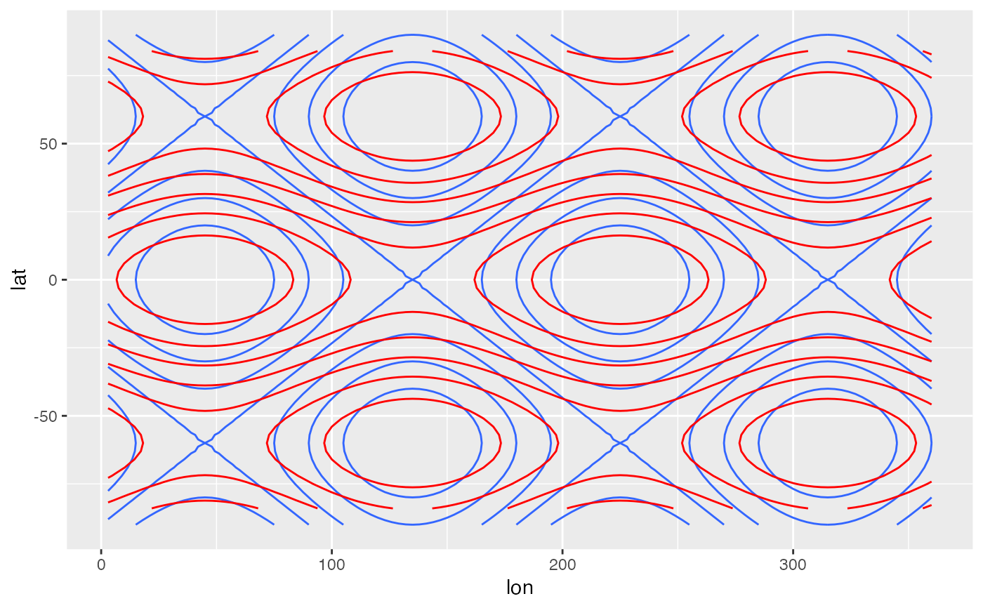
variable <- expand.grid(lon = seq(0, 360, by = 3)[-1],
                        lat = seq(-90, 90, by = 3))
variable$z <- with(variable, cos(lat*pi/180*3) + sin(lon*pi/180*2))
variable <- cbind(
     variable,
     as.data.frame(Derivate(z ~ lon + lat, data = variable,
                          cyclical = c(TRUE, FALSE), order = 2)))
library(ggplot2)
ggplot(variable, aes(lon, lat)) +
    geom_contour(aes(z = z)) +
    geom_contour(aes(z = z.ddlon + z.ddlat), color = "red")
#> Warning: Removed 480 rows containing non-finite values (`stat_contour()`).


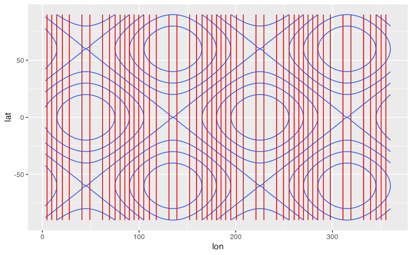
# The same as
ggplot(variable, aes(lon, lat)) +
    geom_contour(aes(z = z)) +
    geom_contour(aes(z = Laplacian(z ~ lon + lat, cyclical = c(TRUE, FALSE))),
                 color = "red")