Aci_fitting

Julien LAMOUR

04/20/2023

Load the R libraries

library(LeafGasExchange)
library(mvtnorm)

Fitting an Aci curve

The objective of this tutorial is to illustrate how to fit an A-Ci curve using the “LeafGasExchange” package. In this tutorial, we first simulate an A-Ci curve with known photosynthetic parameters and noise. This curve is then fitted to retrieve the parameters.

Simulating an Aci curve

For this example we first simulate a photosynthesis curve, but it would work the same if the data were not simulated but measured. The data simulation is done using the function f.A. This function needs a list of photosynthetic parameters which are produced using the function f.make.param() and a list of input variables (CO2 at the surface of the leaf, leaf temperature, incident light, RH). To have more information on the function f.make.param, you can use the command ?f.make.param in R console.

param=f.make.param(VcmaxRef = 50,JmaxRef=50*1.7,TpRef=50/10)
CO2=seq(50,1500,50)
Tleaf=30+273.16
Tair=27+273.16
PAR=1800
RH=80
simul=f.A(PFD = PAR,cs = CO2,Tleaf = Tleaf,Tair = Tair,RH = RH,param = param)

# Here we include a normal error 

simul$A=simul$A+rnorm(n=length(simul$A),mean = 0,sd = 0.6)
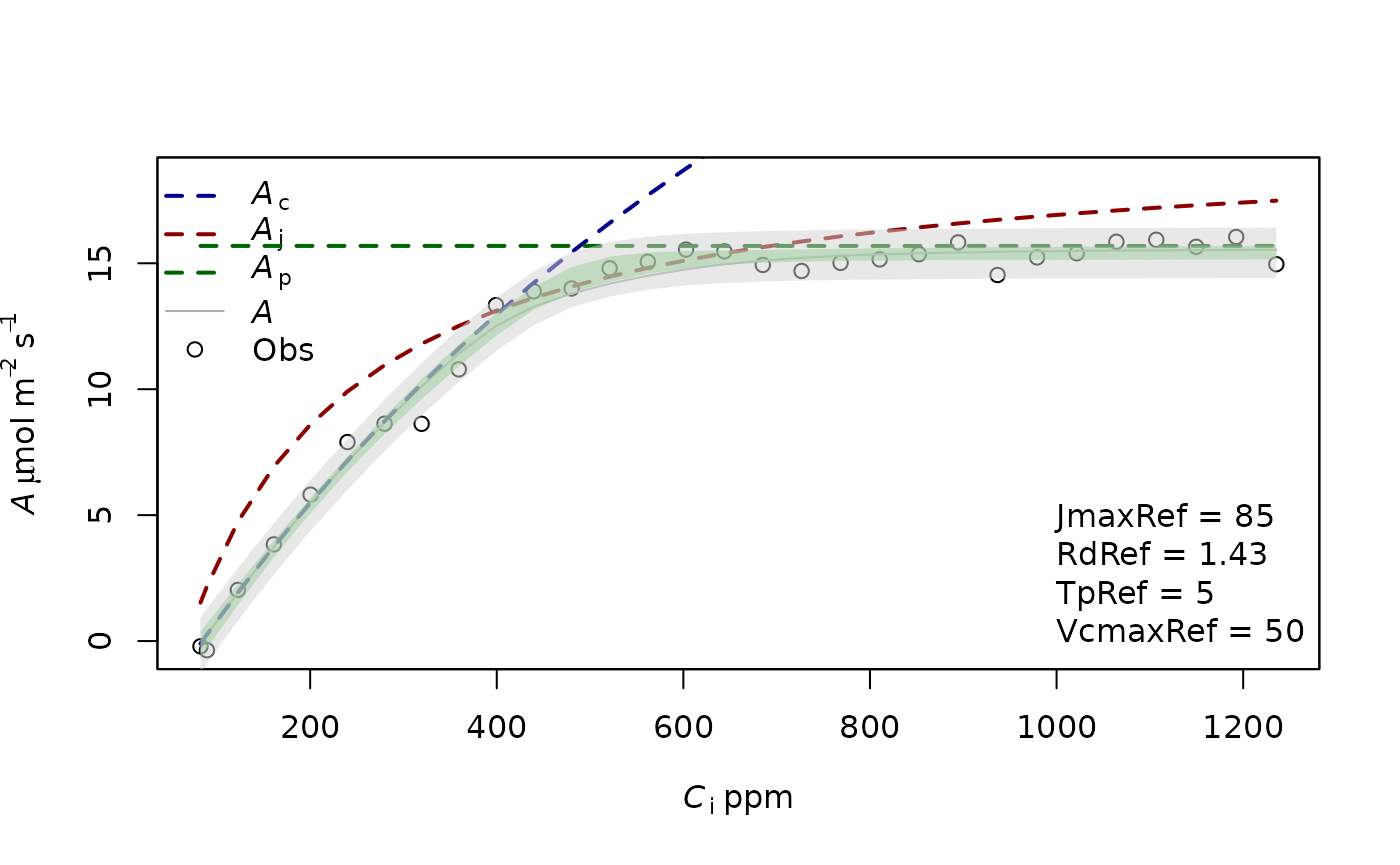
measures=data.frame(Tleaf=Tleaf,Ci=simul$ci,Qin=PAR,A=simul$A)

We display this simulated curve using the function f.plot

f.plot(measures = measures,type = 'Aci',list_legend = param[c('VcmaxRef','JmaxRef','TpRef','RdRef')],param = param)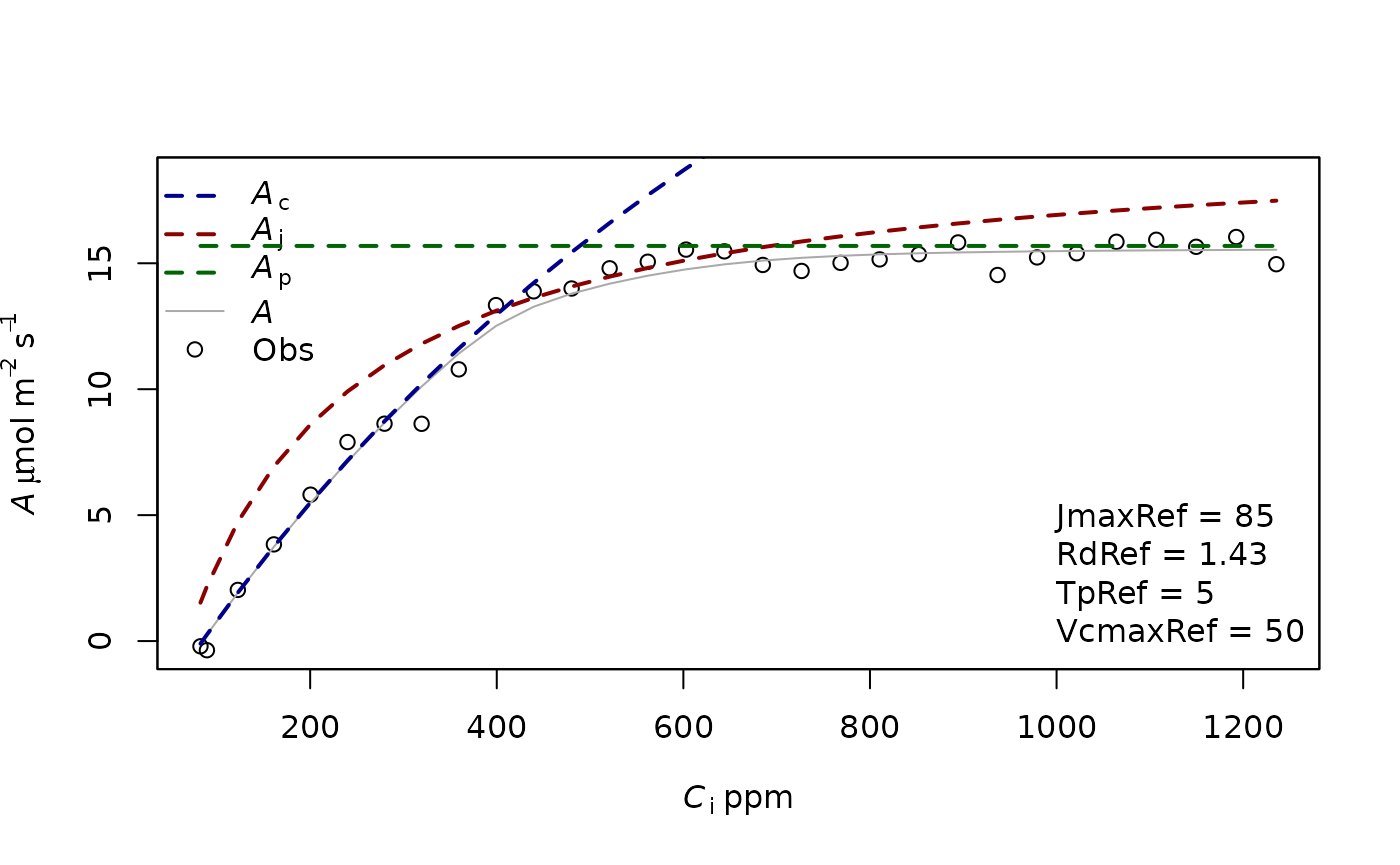

Fitting an Aci curve

To fit an Aci curve, it is necessary to detail the parameter that we want to estimate. All the parameters present in f.make.param can potentially be fitted even if it would not always make sense. We do a first fitting with only the parameters VcmaxRef, JmaxRef and RdRef. Those parameters have to be given in the list Start, with initial values. The method will look for different initial values around those values so it is not necessary to give very good ones, just not too stupid ones. The photosynthetic parameters have to be given in the list param. This is used to determine what should be the parameters for the temperature dependence, for the leaf absorbance, theta, etc. By default, the equations and parameters used in the TBM FATES to simulate the photosynthesis are used. In this example, we also give a very high value to TpRef so the TPU limitation is not considered when fitting the curve.

fitting1=f.fitting(measures = measures,Start = list(JmaxRef = 30, VcmaxRef = 50, RdRef = 1),param=f.make.param(),
                   modify.init=TRUE,do.plot=TRUE,type='Aci')

## $par
##   JmaxRef  VcmaxRef     RdRef 
## 78.962494 47.888017  1.125167 
## 
## $value
## [1] 17.68251
## 
## $counts
## function gradient 
##      216       NA 
## 
## $convergence
## [1] 0
## 
## $message
## NULL
## 
## [1] "sd 0.76773495513519"
## Length  Class   Mode 
##      1   mle2     S4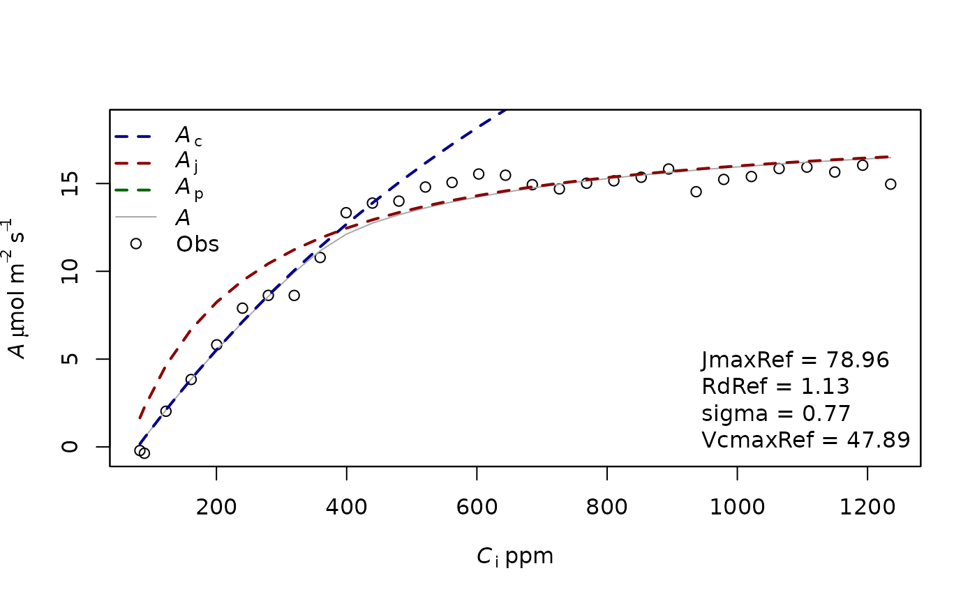

In a second example we now also fit TpRef

fitting2=f.fitting(measures = measures,Start = list(JmaxRef = 30, VcmaxRef = 50, RdRef = 1, TpRef=9),param=f.make.param(),
                   modify.init=TRUE,do.plot=TRUE,type='Aci')

## $par
##   JmaxRef  VcmaxRef     RdRef     TpRef 
## 90.111777 49.634377  1.469053  4.960355 
## 
## $value
## [1] 7.281046
## 
## $counts
## function gradient 
##      369       NA 
## 
## $convergence
## [1] 0
## 
## $message
## NULL
## 
## [1] "sd 0.492647476483964"
## Length  Class   Mode 
##      1   mle2     S4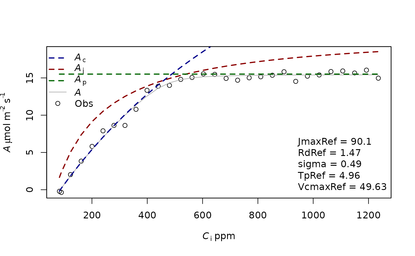

The fitting returns a list of 3 objects. The first object corresponds to the fitting using a minimum square function whereas the second object corresponds to a maximum likelihood derived using the mle2 package. This latter method is useful because it allows us to calculate the confidence interval of the parameters.

The third object correspond to the mean environmental values present in the input data file of the function (see the help of f.fitting for more info).

confint(fitting2[[2]])

##               2.5 %     97.5 %
## sigma     0.3902494  0.6494599
## JmaxRef  84.4848286         NA
## VcmaxRef 46.0850360 53.3552999
## TpRef     4.7420574  5.1695319
## RdRef     0.8935010  2.0412868

It is possible to compare the AIC of the two models using the base function AIC. The lower AIC corresponds to the best model, showing that in this case and as expected, the TPU limitation is useful to improve the fit of the model.

AIC(fitting1[[2]])

## [1] 77.27767

AIC(fitting2[[2]])

## [1] 52.65857

It is also possible to calculate the interval of confidence and prediction of the Aci curve from the outputs of the fitting.

var_cov=fitting2[[2]]@vcov
random_param=rmvnorm(1000,mean=fitting2[[2]]@coef[c('sigma','JmaxRef','VcmaxRef','TpRef','RdRef')],sigma = var_cov)

random_simul=matrix(data = NA,nrow = 1000,ncol = nrow(measures))
for(i in 1:1000){
  random_simul[i,]=f.Aci(PFD = measures$Qin,ci = measures$Ci,Tleaf =measures$Tleaf,param = f.make.param(VcmaxRef=random_param[i,'VcmaxRef'],JmaxRef=random_param[i,'JmaxRef'],TpRef=random_param[i,'TpRef'],
                                                                                                         RdRef=random_param[i,'RdRef']))$A
}

fit_pred=f.Aci(PFD = measures$Qin,ci = measures$Ci,Tleaf =measures$Tleaf,param = f.make.param(VcmaxRef=fitting2[[2]]@coef[c('VcmaxRef')],JmaxRef=fitting2[[2]]@coef[c('JmaxRef')],TpRef=fitting2[[2]]@coef[c('TpRef')],
                                                                                               RdRef=fitting2[[2]]@coef[c('RdRef')]))

sd_mean=apply(X=random_simul,MARGIN=2,FUN=sd)
sd_res=fitting2[[2]]@coef['sigma']
sd_tot=sqrt(sd_mean^2+sd_res^2)
simul_confint=rbind(fit_pred$A-1.96*sd_mean,fit_pred$A+1.96*sd_mean)
simul_pred=rbind(fit_pred$A-1.96*sd_tot,fit_pred$A+1.96*sd_tot)

f.plot(measures = measures,type = 'Aci',list_legend = param[c('VcmaxRef','JmaxRef','TpRef','RdRef')],param = param)
polygon(c(measures$Ci ,rev(measures$Ci)),c(simul_pred[1,], rev(simul_pred[2,])),
        col=adjustcolor("lightgrey",alpha.f=0.5),border=NA)
polygon(c(measures$Ci ,rev(measures$Ci)),c(simul_confint[1,], rev(simul_confint[2,])),
        col=adjustcolor("#99CC99",alpha.f=0.5),border=NA)