Fitting function for photosynthesis data (light curve or Aci curve)

Function to fit model to data. The parameters to fit have to be described in the list Start. All the other parameters of the f.Aci functions have to be in param. If the parameters from Start are repeated in param, the later ones will be ignored. This function uses two methods to fit the data. First by minimizing the residual sum-of-squares of the residuals and then by maximizing the likelihood function. The first method is more robust but the second one allows to calculate the confident interval of the parameters.

f.fitting(
  measures,
  id.name = NULL,
  Start = list(JmaxRef = 90, VcmaxRef = 70, RdRef = 1),
  param = f.make.param(),
  modify.init = TRUE,
  do.plot = TRUE,
  type = "Aci"
)

Arguments

measures: Data frame of measures obtained from gas exchange analyser with at least the columns A, Ci, Qin (the light at the leaf surface in micro mol m-2 s-1) and Tleaf (in K). If RHs, Tair, Patm, VPDleaf are also present, their mean will be added in the output, but those columns are not needed to estimate the parameters.
id.name: Name of the column in the data frame measures with the name for the curve.
Start: List of parameters to fit with their initial values.
param: See f.make.param() for details.
modify.init: TRUE or FALSE, allows to modify the Start values before fitting the data
do.plot: TRUE or FALSE, plot data and fitted curves ?

Value

Return a list with 3 components, 1 the result of the optim function which is used to estimate the parameters, 2 the output of the function bbmle, 3 the mean variable of the environment during the measurement

Examples

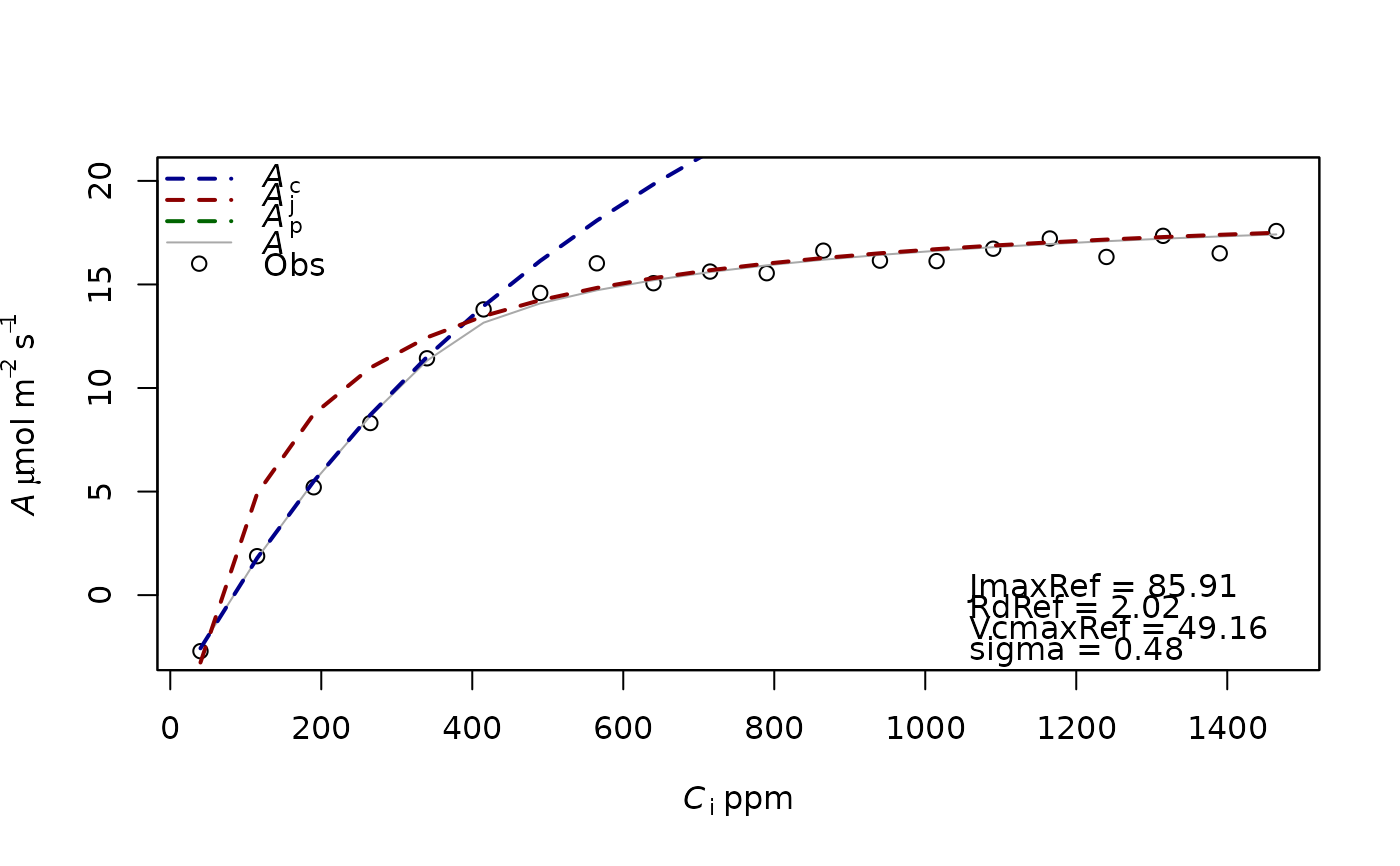
##Simulation of a CO2 curve
data=data.frame(Tleaf=rep(300,20),
Ci=seq(40,1500,75),Qin=rep(2000,20),Tair=300,RHs=70,VPDleaf=2,Patm=101,A=f.Aci(PFD=2000,Tleaf=300,ci=seq(40,1500,75),
param=f.make.param())$A+rnorm(n = 20,mean = 0,sd = 0.5))

f.fitting(measures=data,id.name=NULL,Start=list(JmaxRef=90,VcmaxRef=70,RdRef=1),param=f.make.param())
#> $par
#>  JmaxRef VcmaxRef    RdRef 
#> 85.90353 49.16482  2.02100 
#> 
#> $value
#> [1] 4.629369
#> 
#> $counts
#> function gradient 
#>      146       NA 
#> 
#> $convergence
#> [1] 0
#> 
#> $message
#> NULL
#> 
#> [1] "sd 0.481111694451162"
#> Length  Class   Mode 
#>      1   mle2     S4 

#> [[1]]
#> [[1]]$par
#>  JmaxRef VcmaxRef    RdRef 
#> 85.90353 49.16482  2.02100 
#> 
#> [[1]]$value
#> [1] 4.629369
#> 
#> [[1]]$counts
#> function gradient 
#>      146       NA 
#> 
#> [[1]]$convergence
#> [1] 0
#> 
#> [[1]]$message
#> NULL
#> 
#> 
#> [[2]]
#> 
#> Call:
#> mle2(minuslogl = f.MinusLogL, start = Start, fixed = Fixed, data = list(data = measures))
#> 
#> Coefficients:
#>        sigma            R           O2         TRef         Patm      JmaxRef 
#> 4.811105e-01 8.314000e+00 2.100000e+02 2.981600e+02 1.010000e+02 8.590524e+01 
#>       JmaxHa       JmaxHd        JmaxS     VcmaxRef      VcmaxHa      VcmaxHd 
#> 4.354000e+04 1.520400e+05 4.950000e+02 4.916447e+01 6.533000e+04 1.492500e+05 
#>       VcmaxS        TpRef         TpHa         TpHd          TpS      thetacj 
#> 4.850000e+02 8.333333e+00 5.310000e+04 1.506500e+05 4.900000e+02 9.990000e-01 
#>      thetaip        RdRef         RdHa         RdHd          RdS        KcRef 
#> 9.990000e-01 2.021097e+00 4.639000e+04 1.506500e+05 4.900000e+02 4.049000e+02 
#>         KcHa        KoRef         KoHa     GstarRef      GstarHa         abso 
#> 7.943000e+04 2.784000e+02 3.638000e+04 4.275000e+01 3.783000e+04 8.500000e-01 
#>          aQY        Theta     model.gs           g0           g1        power 
#> 4.250000e-01 7.000000e-01 0.000000e+00 2.000000e-02 4.100000e+00 5.000000e-01 
#> 
#> Log-likelihood: -13.75 
#> 
#> [[3]]
#>    Tair   Tleaf     RHs VPDleaf     Qin    Patm 
#>     300     300      70       2    2000     101 
#>