Computes a linear regression with stats::.lm.fit and returns the estimate and, optionally, standard error for each regressor.
FitLm(y, ..., weights = NULL, se = FALSE, r2 = se)

ResidLm(y, ..., weights = NULL)

Detrend(y, time = seq_along(y))
Arguments
- y
numeric vector of observations to model
- ...
numeric vectors of variables used in the modelling
- weights
numerical vector of weights (which doesn't need to be normalised)
- se
logical indicating whether to compute the standard error
- r2
logical indicating whether to compute r squared
- time
time vector to use for detrending. Only necessary in the case of irregularly sampled timeseries
Value
FitLm returns a list with elements
- term
the name of the regressor
- estimate
estimate of the regression
- std.error
standard error
- df
degrees of freedom
- r.squared
Percent of variance explained by the model (repeated in each term)
- adj.r.squared
r.squared` adjusted based on the degrees of freedom)
ResidLm and Detrend returns a vector of the same length
If there's no complete cases in the regression, NAs are returned with no
warning.
Examples
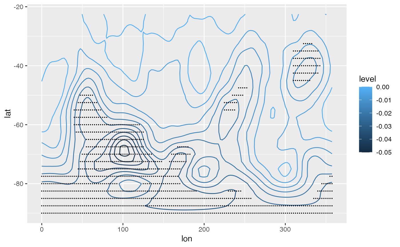
# Linear trend with "signficant" areas shaded with points
library(data.table)
library(ggplot2)
system.time({
  regr <- geopotential[, FitLm(gh, date, se = TRUE), by = .(lon, lat)]
})
#>    user  system elapsed
#>   0.450   0.022   0.476

ggplot(regr[term != "(Intercept)"], aes(lon, lat)) +
    geom_contour(aes(z = estimate, color = ..level..)) +
    stat_subset(aes(subset = abs(estimate) > 2*std.error), size = 0.05)


# Using stats::lm() is much slower and with no names.
if (FALSE) {
system.time({
  regr <- geopotential[, coef(lm(gh ~ date))[2], by = .(lon, lat)]
})
}